用TensorFlow实现戴明回归算法的示例-创新互联

如果最小二乘线性回归算法最小化到回归直线的竖直距离（即，平行于y轴方向），则戴明回归最小化到回归直线的总距离（即，垂直于回归直线）。其最小化x值和y值两个方向的误差，具体的对比图如下图。

创新互联坚持“要么做到，要么别承诺”的工作理念，服务领域包括：成都网站建设、网站建设、企业官网、英文网站、手机端网站、网站推广等服务，满足客户于互联网时代的献县网站设计、移动媒体设计的需求，帮助企业找到有效的互联网解决方案。努力成为您成熟可靠的网络建设合作伙伴！

线性回归算法的损失函数最小化竖直距离；而这里需要最小化总距离。给定直线的斜率和截距，则求解一个点到直线的垂直距离有已知的几何公式。代入几何公式并使TensorFlow最小化距离。

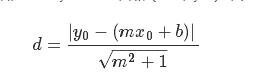
损失函数是由分子和分母组成的几何公式。给定直线y=mx+b，点（x0，y0），则求两者间的距离的公式为：

# 戴明回归
#----------------------------------
#
# This function shows how to use TensorFlow to
# solve linear Deming regression.
# y = Ax + b
#
# We will use the iris data, specifically:
# y = Sepal Length
# x = Petal Width

import matplotlib.pyplot as plt
import numpy as np
import tensorflow as tf
from sklearn import datasets
from tensorflow.python.framework import ops
ops.reset_default_graph()

# Create graph
sess = tf.Session()

# Load the data
# iris.data = [(Sepal Length, Sepal Width, Petal Length, Petal Width)]
iris = datasets.load_iris()
x_vals = np.array([x[3] for x in iris.data])
y_vals = np.array([y[0] for y in iris.data])

# Declare batch size
batch_size = 50

# Initialize placeholders
x_data = tf.placeholder(shape=[None, 1], dtype=tf.float32)
y_target = tf.placeholder(shape=[None, 1], dtype=tf.float32)

# Create variables for linear regression
A = tf.Variable(tf.random_normal(shape=[1,1]))
b = tf.Variable(tf.random_normal(shape=[1,1]))

# Declare model operations
model_output = tf.add(tf.matmul(x_data, A), b)

# Declare Demming loss function
demming_numerator = tf.abs(tf.subtract(y_target, tf.add(tf.matmul(x_data, A), b)))
demming_denominator = tf.sqrt(tf.add(tf.square(A),1))
loss = tf.reduce_mean(tf.truediv(demming_numerator, demming_denominator))

# Declare optimizer
my_opt = tf.train.GradientDescentOptimizer(0.1)
train_step = my_opt.minimize(loss)

# Initialize variables
init = tf.global_variables_initializer()
sess.run(init)

# Training loop
loss_vec = []
for i in range(250):
  rand_index = np.random.choice(len(x_vals), size=batch_size)
  rand_x = np.transpose([x_vals[rand_index]])
  rand_y = np.transpose([y_vals[rand_index]])
  sess.run(train_step, feed_dict={x_data: rand_x, y_target: rand_y})
  temp_loss = sess.run(loss, feed_dict={x_data: rand_x, y_target: rand_y})
  loss_vec.append(temp_loss)
  if (i+1)%50==0:
    print('Step #' + str(i+1) + ' A = ' + str(sess.run(A)) + ' b = ' + str(sess.run(b)))
    print('Loss = ' + str(temp_loss))

# Get the optimal coefficients
[slope] = sess.run(A)
[y_intercept] = sess.run(b)

# Get best fit line
best_fit = []
for i in x_vals:
 best_fit.append(slope*i+y_intercept)

# Plot the result
plt.plot(x_vals, y_vals, 'o', label='Data Points')
plt.plot(x_vals, best_fit, 'r-', label='Best fit line', linewidth=3)
plt.legend(loc='upper left')
plt.title('Sepal Length vs Pedal Width')
plt.xlabel('Pedal Width')
plt.ylabel('Sepal Length')
plt.show()

# Plot loss over time
plt.plot(loss_vec, 'k-')
plt.title('L2 Loss per Generation')
plt.xlabel('Generation')
plt.ylabel('L2 Loss')
plt.show()

网站栏目：用TensorFlow实现戴明回归算法的示例-创新互联
标题路径：https://www.cdcxhl.com/article22/cshcjc.html

成都网站建设公司_创新互联，为您提供关键词优化、商城网站、虚拟主机、网站设计公司、标签优化、电子商务

广告

声明：本网站发布的内容（图片、视频和文字）以用户投稿、用户转载内容为主，如果涉及侵权请尽快告知，我们将会在第一时间删除。文章观点不代表本网站立场，如需处理请联系客服。电话：028-86922220；邮箱：631063699@qq.com。内容未经允许不得转载，或转载时需注明来源： 创新互联